flowchart LR
subgraph Inputs
A["μ"]
B["log σ²"]
end
B --> C["σ = exp(log σ² / 2)"]
D(("ε ~ N(0,1)")) --> E["z = μ + σ·ε"]
C --> E
A --> E
style A fill:#e1f5ff
style B fill:#e1f5ff
style D fill:#fff4e1
style E fill:#e8f5e9
Model
Model initialization and architecture.
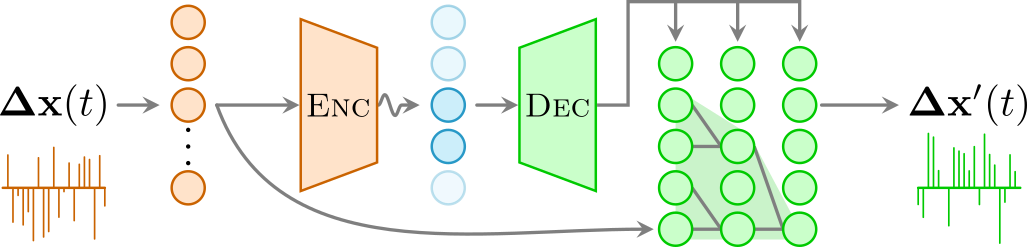
The architecture of the interpretable autoregressive \(\beta\)-VAE works in the following manner: Given the displacements \(\mathbf{\Delta x}(t)\) of a diffusion trajectory, the encoder (orange) compresses them into an interpretable latent space (blue), in which few neurons (dark blue) represent physical features of the input data while others are noised out (light blue). An autoregressive decoder (green) generates from this latent representation the displacements \(\mathbf{\Delta x}'(t)\) of a new trajectory recursively, considering a certain receptive field RF (light green cone).
The models module provides:
- An autoregressive encoder-decoder architecture
VAEWaveNet, implemented as an extension to a convolutional VAEVAEConv1d - Initialization utilities for setting up convolutional layers
- Helper functions for computing output dimensions after convolution operations
After that, we show an example of how to instantiate and train one model.
Initialization
As the architecture can be quite deep, a careful initialization is needed (see weight_init function in the model class). We initialize the weights with normal Kaiming init in fan_out mode, taking into account that we use the nonlinear activation function ReLU.
init_cnn
def init_cnn(
    m:Module, # Module to initialize
):
Initialize module weights with kaiming normal in fan_out mode and bias to 0
VAE
We implement a 1D convolutional variational autoencoder as a base model.
Latent neurons
The latent neurons are probabilistic, i.e., they are sampled following a distribution. The reparameterization trick provides the means to allow backpropagation through these probabilistic neurons by externalizing the sampling noise.
reparameterize
def reparameterize(
    mu:Tensor, # Mean of the normal distribution, shape (batch_size, latent_dim)
    logvar:Tensor, # Diagonal log variance of the normal distribution, shape (batch_size, latent_dim)
)->Tensor: # Sampled latent z, shape (batch_size, latent_dim)
Sample latent tensor using the reparameterization trick: \(z=\epsilon\sigma+\mu\), where \(\epsilon\sim\mathcal{N}(0,1)\).
Output size helpers
We also take into account the sizes after n convolutions are applied to automate the model construction.
output_size_after_n_convt
def output_size_after_n_convt(
    n:int, input_size:int, kernel_size:int, stride:int=1, padding:int=0, output_padding:int=0, dilation:int=1
)->int:
output_size_convt
def output_size_convt(
    input_size:int, kernel_size:int, stride:int=1, padding:int=0, output_padding:int=0, dilation:int=1
)->int:
output_size_after_n_conv
def output_size_after_n_conv(
    n:int, input_size:int, kernel_size:int, stride:int=1, padding:int=0, dilation:int=1
)->int:
output_size_conv
def output_size_conv(
    input_size:int, kernel_size:int, stride:int=1, padding:int=0, dilation:int=1
)->int:
View
def View(
    size:tuple
):
Use as (un)flattening layer
1D Convolutional VAE
VAEConv1d
def VAEConv1d(
    nf:list, # number of filters
    encoder:list, # Encoder's dense layers sizes
    decoder:list, # Decoder's dense layers sizes
    o_dim:int, # input size (T)
    nc_in:int=1, # number of input channels
    nc_out:int=6, # number of output channels
    z_dim:int=6, # number of latent neurons
    beta:float=0.0, # weight of the KLD loss
    avg_size:int=24, # output size of the pooling layers
    kwargs:VAR_KEYWORD
):
1-dimensional convolutional VAE architecture
VAEConv1d Architecture Flow
flowchart LR
    A[Input] --> B[Conv1d]
    subgraph VAEConv1d
    subgraph Encoder
    B --> C[Adaptive<br>Pool<br>& Flatten]
    C --> D[Linear]
    D --> mu["μ"]
    D --> sigma["log σ²"]
    end
    epsilon(("ε ~ N(0,1)")) --> F
    subgraph Latent
    mu --> F["Reparameterize<br>z = μ + σ·ε"]
    sigma --> F
    end
    subgraph Decoder
    F --> G[Linear]
    G --> H[Unflatten &<br>Interpolate]
    H --> I[Conv1d<br>Transpose]
    end
    end
    I --> J[Output]

    style A fill:#e1f5ff
    style F fill:#fff4e1
    style J fill:#e8f5e9
VAE + WaveNet
We extend the VAE with WaveNet as the autoregressive decoder.
sample_from_mix_gaussian
def sample_from_mix_gaussian(
    y:Tensor, # Mixture of Gaussians parameters. Shape (B x C x T)
    log_scale_min:float=-12.0, # Log scale minimum value.
)->Tensor:
Sample from (discretized) mixture of gaussian distributions.
DilatedCausalConv1d
def DilatedCausalConv1d(
    mask_type:str, in_channels:int, out_channels:int, kernel_size:int=2, dilation:int=1, bias:bool=True,
    use_pad:bool=True
):
Dilated causal convolution for WaveNet
ResidualBlock
def ResidualBlock(
    res_channels:int, skip_channels:int, kernel_size:int, dilation:int, c_channels:int=0, g_channels:int=0,
    bias:bool=True, use_pad:bool=True
):
Residual block with conditions and gate mechanism
ResidualBlock Architecture Flow
flowchart LR
    C[Local<br>Conditioning<br>c] --> D[Conv1d 1x1]-->C2[Chunk]-->c1-->sum1
    C2-->c2-->sum2
    A[Input<br>x] --> B[Dilated<br>Causal<br>Conv1d]-->Chunk-->o1-->sum1[+]
    Chunk-->o2-->sum2[+]
    sum2 --> H
    sum1 --> G
    subgraph Gated Activation
        H[sigmoid]-->*
        G["id #tanh"]-->*
    end
    * --> K[Conv1d 1x1] --> N[Skip<br>Output]
    * --> J[Conv1d 1x1] --> L[+] --> M[Residual<br>Output]
    A --> L

    style A fill:#e1f5ff
    style C fill:#e1f5ff
    style M fill:#e8f5e9
    style N fill:#fff4e1
VAEWaveNet
def VAEWaveNet(
    in_channels:int=1, # input channels
    res_channels:int=16, # residual block channels
    skip_channels:int=16, # skip connection channels
    c_channels:int=6, # local conditioning (time-wise)
    g_channels:int=0, # global conditioning (the same for the whole sequence)
    out_channels:int=1, # output channels
    res_kernel_size:int=3, # kernel_size of dilated layers in residual blocks
    layer_size:int=4, # largest dilation is 2^layer_size
    stack_size:int=1, # number of layers stacks
    out_distribution:str='normal', discrete_channels:int=256, num_mixtures:int=1, # 1=no mixture
    use_pad:bool=False, weight_norm:bool=False, kwargs:VAR_KEYWORD
):
VAE with autoregressive decoder
VAEWaveNet Architecture Flow
flowchart LR
    A[Input<br>x] --> B[VAEConv1d] --> C[Local<br>Conditioning<br>c]-->W[WaveNet]
    A-->W[WaveNet]-->O[Output<br>Probability]
WaveNet Architecture Flow
flowchart LR
    C[Local<br>Conditioning<br>c] --> R
    C-.->R2
    C-->R3
    A[Input<br>x] --> B[Conv1d 1x1]--> D[Dilated<br>Causal<br>Conv1d]--> R[Residual<br>Block]
    subgraph RS["Residual Stack"]
    R -.-> R2["···"] -.-> R3[Residual<br>Block]
    end
    R  --> s1
    R2 -.-> s2
    R3 --> s3
    %% the plus sign alone is interpreted as markdown list, thus #43;
    S["Skip=0"] -->s1(("#43;"))-.->s2(("#43;"))-.->s3(("#43;"))-->Conv1d-->O[Output]
We can create a model by specifying its parameters in a dict.
model_args = dict(# VAE #########################
                  o_dim=400,
                  nc_in=1, nc_out=6,
                  nf=[16]*4,
                  avg_size=16,
                  encoder=[200,100],
                  z_dim=6,
                  decoder=[100,200],
                  beta=0,
                  # WaveNet ########
                  in_channels=1,
                  res_channels=16,skip_channels=16,
                  c_channels=6,
                  g_channels=0,
                  res_kernel_size=3,
                  layer_size=4,  # 6
                  stack_size=1,
                  out_distribution= "Normal",
                  num_mixtures=1,
                  use_pad=False,
                  model_name = 'SPIVAE',
                 )
model = VAEWaveNet(**model_args)
Printing the model object will reveal the declared layers.
modelVAEWaveNet(
(vae): VAEConv1d(
(encoder): Sequential(
(0): Conv1d(1, 16, kernel_size=(3,), stride=(1,))
(1): ReLU(inplace=True)
(2): Conv1d(16, 16, kernel_size=(3,), stride=(1,))
(3): ReLU(inplace=True)
(4): Conv1d(16, 16, kernel_size=(3,), stride=(1,))
(5): ReLU(inplace=True)
(6): Conv1d(16, 16, kernel_size=(3,), stride=(1,))
(7): ReLU(inplace=True)
(8): AdaptiveConcatPool1d(
(ap): AdaptiveAvgPool1d(output_size=16)
(mp): AdaptiveMaxPool1d(output_size=16)
)
(9): View()
(10): Linear(in_features=512, out_features=200, bias=True)
(11): ReLU(inplace=True)
(12): Linear(in_features=200, out_features=100, bias=True)
(13): ReLU(inplace=True)
(14): Linear(in_features=100, out_features=12, bias=True)
)
(decoder): Sequential(
(0): Linear(in_features=6, out_features=100, bias=True)
(1): ReLU(inplace=True)
(2): Linear(in_features=100, out_features=200, bias=True)
(3): ReLU(inplace=True)
(4): Linear(in_features=200, out_features=512, bias=True)
(5): ReLU(inplace=True)
(6): View()
)
(convt): Sequential(
(0): ConvTranspose1d(16, 16, kernel_size=(3,), stride=(1,))
(1): ReLU(inplace=True)
(2): ConvTranspose1d(16, 16, kernel_size=(3,), stride=(1,))
(3): ReLU(inplace=True)
(4): ConvTranspose1d(16, 16, kernel_size=(3,), stride=(1,))
(5): ReLU(inplace=True)
(6): ConvTranspose1d(16, 6, kernel_size=(3,), stride=(1,))
(7): ReLU(inplace=True)
)
)
(init_conv): Conv1d(1, 16, kernel_size=(1,), stride=(1,))
(causal): DilatedCausalConv1d(
(conv): Conv1d(16, 16, kernel_size=(2,), stride=(1,))
)
(res_stack): ModuleList(
(0): ResidualBlock(
(dilated): DilatedCausalConv1d(
(conv): Conv1d(16, 32, kernel_size=(3,), stride=(1,))
)
(conv_c): Conv1d(6, 32, kernel_size=(1,), stride=(1,), bias=False)
(conv_res): Conv1d(16, 16, kernel_size=(1,), stride=(1,))
(conv_skip): Conv1d(16, 16, kernel_size=(1,), stride=(1,))
)
(1): ResidualBlock(
(dilated): DilatedCausalConv1d(
(conv): Conv1d(16, 32, kernel_size=(3,), stride=(1,), dilation=(2,))
)
(conv_c): Conv1d(6, 32, kernel_size=(1,), stride=(1,), bias=False)
(conv_res): Conv1d(16, 16, kernel_size=(1,), stride=(1,))
(conv_skip): Conv1d(16, 16, kernel_size=(1,), stride=(1,))
)
(2): ResidualBlock(
(dilated): DilatedCausalConv1d(
(conv): Conv1d(16, 32, kernel_size=(3,), stride=(1,), dilation=(4,))
)
(conv_c): Conv1d(6, 32, kernel_size=(1,), stride=(1,), bias=False)
(conv_res): Conv1d(16, 16, kernel_size=(1,), stride=(1,))
(conv_skip): Conv1d(16, 16, kernel_size=(1,), stride=(1,))
)
(3): ResidualBlock(
(dilated): DilatedCausalConv1d(
(conv): Conv1d(16, 32, kernel_size=(3,), stride=(1,), dilation=(8,))
)
(conv_c): Conv1d(6, 32, kernel_size=(1,), stride=(1,), bias=False)
(conv_res): Conv1d(16, 16, kernel_size=(1,), stride=(1,))
(conv_skip): Conv1d(16, 16, kernel_size=(1,), stride=(1,))
)
)
(out_conv): Sequential(
(0): ReLU(inplace=True)
(1): Conv1d(16, 16, kernel_size=(1,), stride=(1,))
(2): ReLU(inplace=True)
(3): Conv1d(16, 9, kernel_size=(1,), stride=(1,))
)
)Training a VAEWaveNet
The following example demonstrates a complete training workflow: loading data, initializing the model, and training with fastai’s Learner.
DEVICE= 'cpu' # 'cuda'
print(DEVICE)cpuN=6_000Ds = np.linspace(2e-5,2e-2,5)
alphas = np.linspace(0.2,1.8,9)
n_alphas,n_Ds = len(alphas), len(Ds)
ds_args = dict(path="../../data/raw/", model='fbm', # 'sbm'
N=int(N/n_alphas/n_Ds*2), T=400,
D=Ds, alpha=alphas,seed=0,
valid_pct=0.2, bs=2**8,
N_save=N, T_save=400,
)model_args = dict(# VAE ###########################
o_dim=ds_args['T']-1,
nc_in=1, nc_out=6,
nf=[16]*4,
avg_size=16,
encoder=[200,100],
z_dim=6,
decoder=[100,200],
beta=0,
# WaveNet ########
in_channels=1,
res_channels=16,skip_channels=16,
c_channels=6,
g_channels=0,
res_kernel_size=3,
layer_size=4, # 6 # Largest dilation is 2**layer_size
stack_size=1,
out_distribution= "Normal",
num_mixtures=1,
use_pad=False,
model_name = 'SPIVAE',
)dls = load_data(ds_args)model = VAEWaveNet(**model_args).to(DEVICE)loss_fn = Loss(model.receptive_field, model.c_channels,
beta=model_args['beta'], reduction='mean')learn = Learner(dls, model, loss_func=loss_fn,)E=4learn.fit_one_cycle(E, lr_max=1e-4)| epoch | train_loss | valid_loss | time |
|---|---|---|---|
| 0 | 0.982180 | 0.949590 | 00:28 |
| 1 | 0.934559 | 0.880010 | 00:25 |
| 2 | 0.882010 | 0.822553 | 00:26 |
| 3 | 0.843744 | 0.810182 | 00:29 |