Data

Data generation, preprocessing, and loading.

The data module provides:

Trajectory generators for stochastic processes from the andi_datasets library.
The load_data function that bundles preprocessing, splitting, and batching into a single call, ready for training.

Both parts are exemplified for the fractional Brownian motion and scaled Brownian motion datasets.

flowchart LR
    A["FBM<br>AD.create_datasets()"] --> Disk[(fbm.h5)]
    B["SBM<br>sbm()"] --> Disk2[(sbm.npz)]
    C[ds_args] --> E["load_data()"]
    Disk --> E
    Disk2 --> E
    E --> F[Preprocess]
    F --> G[Train/Val<br>Split]
    subgraph J["DataLoaders dls"]
        H[Training<br>DataLoader<br>dls.train]
        I[Validation<br>DataLoader<br>dls.valid]
    end
    G --> H
    G --> I
    style Disk fill:#e1f5ff
    style Disk2 fill:#e1f5ff
    style E fill:#fff4e1
    style H fill:#e8f5e9
    style I fill:#e8f5e9

Data generation

To study stochastic processes, we take trajectories from three paradigmatic diffusion models: Brownian motion, fractional Brownian motion, and scaled Brownian motion.

We generate the trajectories with the andi_datasets package.

Fractional Brownian motion

For fractional Brownian motion (FBM), we take \(\alpha\in[0.04, 1.96]\). For the dataset of Brownian motion (BM), we can take directly the FBM trajectories with \(\alpha=1\).

alphas_train = np.linspace(0.2,1.8,21)
alphas_test  = np.linspace(0.04,1.96,49)
print(f'{alphas_train=}')
print(f'{alphas_test=}')

alphas_train=array([0.2 , 0.28, 0.36, 0.44, 0.52, 0.6 , 0.68, 0.76, 0.84, 0.92, 1.  ,
       1.08, 1.16, 1.24, 1.32, 1.4 , 1.48, 1.56, 1.64, 1.72, 1.8 ])
alphas_test=array([0.04, 0.08, 0.12, 0.16, 0.2 , 0.24, 0.28, 0.32, 0.36, 0.4 , 0.44,
       0.48, 0.52, 0.56, 0.6 , 0.64, 0.68, 0.72, 0.76, 0.8 , 0.84, 0.88,
       0.92, 0.96, 1.  , 1.04, 1.08, 1.12, 1.16, 1.2 , 1.24, 1.28, 1.32,
       1.36, 1.4 , 1.44, 1.48, 1.52, 1.56, 1.6 , 1.64, 1.68, 1.72, 1.76,
       1.8 , 1.84, 1.88, 1.92, 1.96])

As advised in the andi_datasets library, we can save at the beginning a big dataset of long (T_save \(\sim 10^3\)) and numerous (N_save \(\sim 10^4\)) trajectories which then allows us to load any other combination of T and N_models.

AD.avail_models_name

['attm', 'ctrw', 'fbm', 'lw', 'sbm']

N=6_000 # number of trajectories per parameter combination

T=400
dataset = AD.create_dataset(T=T, N_models=N,
                            exponents=alphas_test,
                            models=[2],   # fbm
                            dimension=1,
                            N_save=N,
                            T_save=T,
                            save_trajectories=True,
                            load_trajectories=False, # False allows saving
                            path="../../data/raw/")

The andi_datasets gives us the trajectories with shape \([N*|\mathrm{exponents}|, 2+T]\) where the first two data points of each vector are the model label and the anomalous exponent \(\alpha\).

dataset.shape, dataset[0,:2], dataset[-1,:2]

((294000, 402), array([2.  , 0.04]), array([2.  , 1.96]))

The following \(T\) points compose the trajectory that always has zero origin.

Show/hide code

plt.plot(dataset[0,2:], label=f'{alphas_test[0]:.3g}');
plt.plot(dataset[49//2*N,2:], label=f'{alphas_test[49//2]:.3g}');
plt.plot(dataset[-1,2:], label=f'{alphas_test[-1]:.3g}');
plt.xlabel(r'$t$');plt.ylabel(r'$x$', rotation=0);
plt.legend(title=r'$\alpha$');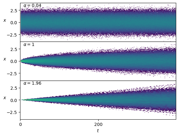

The distribution of the positions \(x(t)\) depends on \(\alpha\) and time, as we expect from the mean squared displacement relation \(\langle x^2\rangle=2 D t^\alpha\).

Show/hide code

fig, axs = plt.subplots(3,1, sharex=True, gridspec_kw=dict(hspace=0))
for ax, a_i in zip(axs,[0,49//2,48]):
    ax.hist2d(np.tile(np.arange(T),N),dataset[a_i*N:(a_i+1)*N,2:].reshape(-1), T, cmin=2, norm=matplotlib.colors.LogNorm());
    ax.text(0.02,0.9, r'$\alpha=' f'{dataset[a_i*N,1]:.3g}' r'$', transform=ax.transAxes);
    ax.set_ylabel(r'$x$', rotation=0);
    ax.set_ylim([-4,4])
    ax.locator_params(nbins=3);
axs[-1].set_xlabel(r'$t$');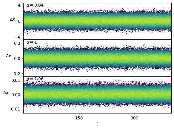

Conveniently, the displacements \(\Delta x\) are stationary.

Show/hide code

fig, axs = plt.subplots(3,1, sharex=True, gridspec_kw=dict(hspace=0))
for ax, a_i in zip(axs,[0,49//2,48]):
    ax.hist2d(np.tile(np.arange(T-1),N),np.subtract(dataset[a_i*N:(a_i+1)*N,3:],dataset[a_i*N:(a_i+1)*N,2:-1]).reshape(-1), T-1, cmin=2, norm=matplotlib.colors.LogNorm());
    ax.text(0.02,0.9, r'$\alpha=' f'{dataset[a_i*N,1]:.3g}' r'$', transform=ax.transAxes);
axs[-1].set_xlabel(r'$t$');
for ax in axs : ax.set_ylabel(r'$\Delta x$', rotation=0);

Scaled Brownian motion

For the generation of scaled Brownian motion (SBM) trajectories, we take the generating function from andi_datasets to control sigma as \(D_0\) and generate displacements directly.

source

sbm


def sbm(
    T:int, # trajectory time steps
    alpha:float, sigma:float=1.0
)->array:

Creates T scaled Brownian motion displacements.

We select the range of values to coincide with the previous dataset.

N=1_000

T=400
Ds = np.geomspace(1e-5,1e-2, 10)
alphas_train = np.linspace(0.2,1.8,21)

disp = {f'{a:.3g}'+f',{D:.3g}':[] for D in Ds for a in alphas_train}
fname = '../../data/raw/sbm.npz'
if not os.path.exists(fname):  # create
    for i,a in enumerate(alphas_train):
        for j,D in enumerate(Ds):
            k = f'{a:.3g}'+f',{D:.3g}'
            disp[k]=np.array([np.concatenate(([a,D],sbm(T, a, sigma = D2sig(D)))) for n in range(N)]) # N, T+2
    np.savez_compressed(fname,**disp)
    print('Saved at:', fname)
else:  # load
    with np.load(fname) as f:
        for i,a in enumerate(alphas_train):
            for j,D in enumerate(Ds):
                k = f'{a:.3g}'+f',{D:.3g}'
                disp[k] = f[k][:N,:2+T]
    print('Loaded from:', fname)

Loaded from: ../../data/raw/sbm.npz

The displacements follow the temporal scaling \(D_\alpha(t) = \alpha D_0 t^{\alpha-1}\).

Show/hide code

fig, axs = plt.subplots(3,1, sharex=True, gridspec_kw=dict(hspace=0))
for ax, a in zip(axs,[0.2,1,1.8]):
    k = f'{a:.3g}'+f',0.01'
    ax.hist2d(np.tile(np.arange(T),N),disp[k][:,2:].reshape(-1), T, cmin=2, norm=matplotlib.colors.LogNorm());
    ax.text(0.02,0.9, r'$\alpha=' f'{a:.3g}' r'$', transform=ax.transAxes);
    ax.set_ylabel(r'$\Delta x$', rotation=0);
axs[-1].set_xlabel(r'$t$');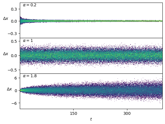

We can do the same to create a test set.

Ds = np.geomspace(1e-6,1e-1,16)[2:-2] # np.geomspace(1e-6,1e-1,61)[6:-6]
alphas = np.linspace(0.04,1.96,49)
disp_test = {f'{a:.3g}'+f',{D:.3g}':[] for D in Ds for a in alphas_train}
fname = '../../data/test/sbm.npz'
if not os.path.exists(fname):  # create
    os.makedirs('../../data/test/', exist_ok=True)
    for i,a in enumerate(alphas_train):
        for j,D in enumerate(Ds):
            k = f'{a:.3g}'+f',{D:.3g}'
            disp_test[k]=np.array([np.concatenate(([a,D],sbm(T, a, sigma = D2sig(D)))) for n in range(N)]) # N, T+2
    np.savez_compressed(fname,**disp_test)
    print('Saved at:', fname)

Data Loader

To load trajectories, we use the convenience funtion load_data(). This function accepts a configuration dictionary and returns the fastai DataLoaders object. This object takes care of the splitting and preprocessing of the data, as well as shuffling batches in training and some other utilities.

To select the dataset, the function expects a ds_args dictionary with the following structure:

ds_args = {
    'path': str,              # Data directory path
    'model': 'fbm' or 'sbm',  # Process type
    'alpha': list[float],     # Exponent values
    'D': list[float],         # Diffusion coefficients
    'T': int,                 # Trajectory length
    'N': int,                 # Number of trajectories per parameter
    'N_save': int,            # Total saved trajectories
    'T_save': int,            # Saved trajectory length
    'valid_pct': float,       # Validation split percentage
    'seed': int,              # Random seed
    'bs': int,                # Batch size
}

source

ConditionalsTransform


def ConditionalsTransform(
    n_labels:int=1
):

Extracts the positional information from the input array, inserts a channel dimension for convolutions, and discards the labels.

source

load_data


def load_data(
    ds_args:dict
)->DataLoaders:

Loads a dataset from the given args and returns train and validation DataLoaders. Trajectories are preprocessed on load and on-the-fly via ConditionalsTransform.

Visualization helpers

The following functions provide standardized plots for inspecting generated trajectories and their statistical properties. They are used throughout the tutorials to verify that generated data behaves as expected.

source

set_plot_xf


def set_plot_xf(
    x_label:str='', y_label:str='', title:str='', x_scale:str='linear', y_scale:str='linear', legend_title:str='',
    save:bool=False, ncol:int=1, show_legend:bool=True
):

Configure axis labels and formatting for trajectory plots.

source

plot_xf_D


def plot_xf_D(
    x, f, ds_args:dict, intersect_idx, f_a:NoneType=None, f_D:NoneType=None, f_aD:NoneType=None, each_D:bool=True,
    each_g:bool=True, kwargs:VAR_KEYWORD
):

Plots f(x) using the provided indices and auxiliary functions

source

f_a_text


def f_a_text(
    a, y
):

Format an anomalous exponent a value as a text annotation in (0.95,y) of axes coordinates

source

plot_xf


def plot_xf(
    x, f, ds_args:dict, intersect_idx, x_label:str='', y_label:str='', title:str='', x_scale:str='linear',
    y_scale:str='linear'
):

Plot a set of input arrays x transformed by f and colored by a parameter combination.

FBM

To load the dataset of FBM, we simply specify the dataset parameters in a dict and call load_data with it.

N=6_000; bs=2**8

Ds     = [1e-4, 1e-3, 1e-2]
alphas = [0.6, 1.0, 1.4]
n_alphas, n_Ds = len(alphas), len(Ds)
ds_args = dict(path="../../data/raw/", model='fbm', # 'sbm'
               D=Ds, alpha=alphas,
               N=int(N/n_alphas/n_Ds), T=400,
               N_save=N, T_save=400,
               seed=0, valid_pct=0.2, bs=bs,
              )
dls = load_data(ds_args)

Once loaded, we can inspect the data that bring the DataLoaders.

print(dls.bs, dls.device, len(dls.one_batch()))
print(L(map(lambda x: x.shape, dls.one_batch())))
#print(dls.one_batch())

256 cpu 2
[torch.Size([256, 1, 399]), torch.Size([256, 399, 1])]

alphas_items = dls.valid.items[:,0]
Ds_items     = dls.valid.items[:,1]
ds_in_labels = dls.valid.items[:,:2]
u_a=np.unique(alphas_items,)
u_D=np.unique(Ds_items,)
alphas_idx = [np.flatnonzero(alphas_items==a) for a in u_a]
Ds_idx = [np.flatnonzero(Ds_items==D) for D in u_D]
intersect_idx = np.array([[reduce(partial(np.intersect1d,assume_unique=True),
                                       (alphas_idx[i],Ds_idx[j]))
                                for j,D in enumerate(u_D)] for i,a in enumerate(u_a)], dtype=object)

We fetch the preprocessed dataset as the model will see in the following loop.

ds_in = []
with torch.no_grad():
    for b in tqdm(dls.valid):
        x,y=b
        ds_in.append(to_detach(x).numpy())
ds_in = np.concatenate(ds_in)
print(ds_in.shape)

(1198, 1, 399)

The samples are the displacements \(\Delta x\) of a trajectory.

Show/hide code

plt.plot(ds_in.squeeze()[:2].T); plt.xlabel(r'$t$'); plt.ylabel(r'$\Delta x$', rotation=0);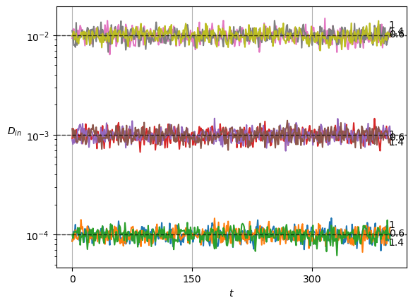

FBM displacements follow a Gaussian distribution \(\mathcal{N}(\mu, \sigma^2)\) which is centered at \(\mu=0\) and whose variance is related to the diffusion coefficient as \(\sigma^2 = 2D\).

Show/hide code

for i,D in enumerate(u_D): plt.hist(ds_in[Ds_idx[i]].reshape(-1),500, histtype='step', label=f'{D:.2g}');
plt.ylabel('Counts'); plt.xlabel(r'$\Delta x$'); plt.legend(title=r'$D$');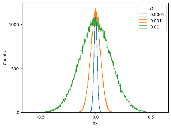

Therefore, the mean and variance of the displacements constitute two straightforward sanity checks that the generated displacements must satisfy.

Show/hide code

plot_xf(ds_in, lambda x: x.squeeze().mean(0),ds_args, intersect_idx, x_label=r'$t$', y_label=r'$\mu_{in}$',)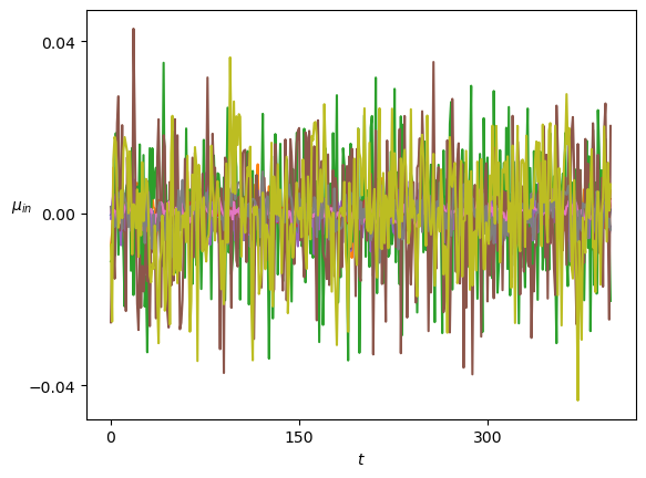

Show/hide code

plot_xf_D(ds_in, lambda x: sig2D(x.squeeze().std(0)),ds_args, intersect_idx,
          f_a=f_a_text,
          f_D=lambda D: plt.axhline(D, c='k', lw=1, ls='--', alpha=0.7),
          each_D=False,each_g=False, x_label=r'$t$', y_label=r'$D_{in}$',
          y_scale='log', show_legend=False,
         )

SBM

Similarly, to load the dataset of SBM, we simply specify the dataset parameters in a dict and call load_data with it.

N=1_000

Ds = [1e-5,1e-4,1e-3, 1e-2]  # np.geomspace(1e-5,1e-2, 10)
alphas = np.linspace(0.2,1.8,21)
n_alphas, n_Ds = len(alphas), len(Ds)
ds_args = dict(path="../../data/raw/", model='sbm',
               N=int(N/n_alphas/n_Ds), T=400,
               D=Ds, alpha=alphas,
               N_save=N, T_save=400,
               seed=0, valid_pct=0.8, bs=2**8,)

dls = load_data(ds_args)

As we did before, we can inspect the data that brings the DataLoaders.

alphas_items = dls.valid.items[:,0]
Ds_items     = dls.valid.items[:,1]
ds_in_labels = dls.valid.items[:,:2]
u_a=np.unique(alphas_items,)
u_D=np.unique(Ds_items,)
alphas_idx = [np.flatnonzero(alphas_items==a) for a in u_a]
Ds_idx = [np.flatnonzero(Ds_items==D) for D in u_D]
intersect_idx = np.array([[reduce(partial(np.intersect1d,assume_unique=True),
                                       (alphas_idx[i],Ds_idx[j]))
                                for j,D in enumerate(u_D)] for i,a in enumerate(u_a)], dtype=object)

ds_in = []
with torch.no_grad():
    for b in tqdm(dls.valid):
        x,y=b
        ds_in.append(to_detach(x).numpy())
ds_in = np.concatenate(ds_in)
print(ds_in.shape)

(9996, 1, 399)

SBM displacements have a zero mean but follow the scaling of the aging diffusion coefficient \(D_\alpha (t) = \alpha D_0 t^{\alpha-1}\).

Show/hide code

plt.plot(ds_in.squeeze()[:2].T); plt.xlabel(r'$t$'); plt.ylabel(r'$\Delta x$', rotation=0);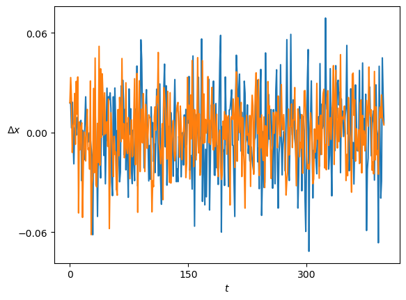

For \(\alpha<1\), the displacements become smaller as time passes. On the contrary, \(\alpha>1\) leads to a growth of the displacements.

Show/hide code

fig, axs = plt.subplots(3,1, sharex=True, gridspec_kw=dict(hspace=0))
for ax, a_i in zip(axs,[0,n_alphas//2,n_alphas-1]):
    x = ds_in.squeeze()[alphas_idx[a_i]]
    ax.hist2d(np.tile(np.arange(x.shape[-1]),x.shape[0]),x.reshape(-1),x.shape[-1],
              cmin=2, norm=matplotlib.colors.LogNorm());
    ax.text(0.02,0.9, r'$\alpha=' f'{u_a[a_i]:.3g}' r'$', transform=ax.transAxes);
    ax.set_ylabel(r'$\Delta x$', rotation=0);
axs[-1].set_xlabel(r'$t$');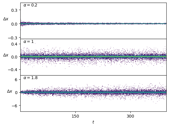

We plot the means of the displacements.

Show/hide code

plot_xf(ds_in, lambda x: x.squeeze().mean(0),ds_args, intersect_idx, x_label=r'$t$', y_label=r'$\mu_{in}$',)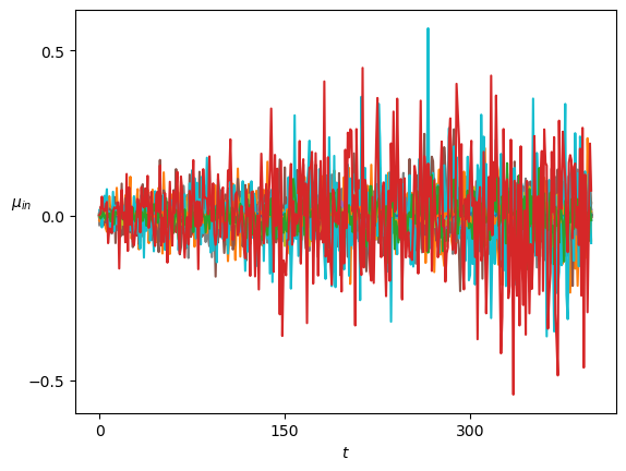

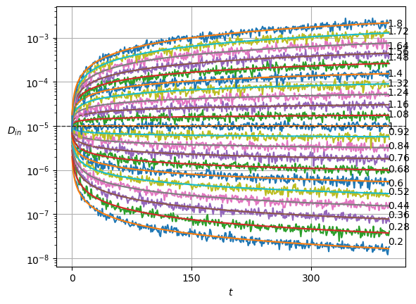
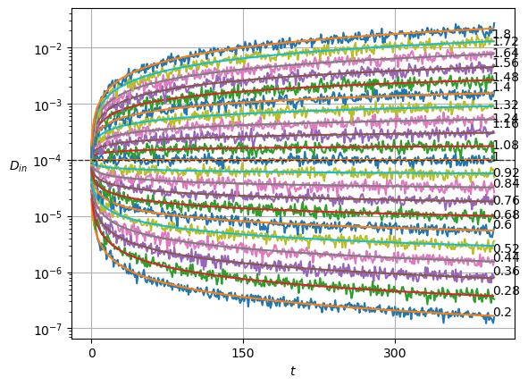
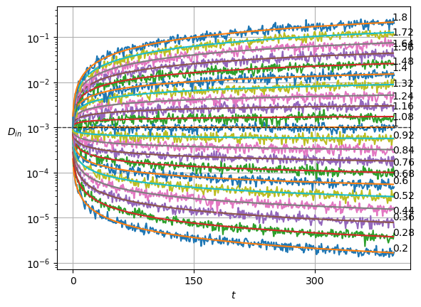
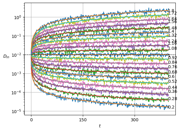
In SBM, each \(\alpha\) is shown in the variance at each time step. Thus, this simple sanity check is now a direct observation of the displacements properties.

Show/hide code

x = ds_in.squeeze()
plot_xf_D(x, lambda x: sig2D(x.squeeze().std(0)),ds_args, intersect_idx,
          f_a=lambda a,y: plt.text(0.95,y[-1],f'{a:.3g}', transform=matplotlib.transforms.blended_transform_factory(plt.gca().transAxes, plt.gca().transData)),
          f_D=lambda D: plt.axhline(D, c='k', lw=1, ls='--', alpha=0.7),
          f_aD=lambda a,D: plt.plot(a*D*np.arange(1,x.shape[-1])**(a-1.)),
          each_D=True,each_g=False, x_label=r'$t$', y_label=r'$D_{in}$',
          y_scale='log', show_legend=False,
         )